Huaxia Wang
Department of Electrical and Computer Engineering
Stevens Institute of Technology
Hoboken, NJ 07030, USA
hwang38@stevens.edu
&Chun-Nam Yu
Nokia Bell Labs
600 Mountain Avenue
Murray Hill, NJ 07974, USA
chun-nam.yu@nokia-bell-labs.com
Deep neural networks have been shown to perform well in many classical machine learning problems, especially in image classification tasks. However, researchers have found that neural networks can be easily fooled, and they are surprisingly sensitive to small perturbations imperceptible to humans. Carefully crafted input images (adversarial examples) can force a well-trained neural network to provide arbitrary outputs. Including adversarial examples during training is a popular defense mechanism against adversarial attacks. In this paper we propose a new defensive mechanism under the generative adversarial network (GAN) framework. We model the adversarial noise using a generative network, trained jointly with a classification discriminative network as a minimax game. We show empirically that our adversarial network approach works well against black box attacks, with performance on par with state-of-art methods such as ensemble adversarial training and adversarial training with projected gradient descent.
Deep neural networks have been successfully applied to a variety of tasks, including image classification (Krizhevsky et al., 2012) , speech recognition (Graves et al., 2013) , and human-level playing of video games through deep reinforcement learning (Mnih et al., 2015) . However, Szegedy et al. (2014) showed that convolutional neural networks (CNN) are extremely sensitive to carefully crafted small perturbations added to the input images. Since then, many adversarial examples generating methods have been proposed, including Jacobian based saliency map attack (JSMA) (Papernot et al., 2016a) , projected gradient descent (PGD) attack (Madry et al., 2018) , and C & \& W’s attack (Carlini & Wagner, 2017) . In general, there are two types of attack models: white box attack and black box attack. Attackers in white box attack model have complete knowledge of the target network, including network’s architecture and parameters. Whereas in black box attacks, attackers only have partial or no information on the target network (Papernot et al., 2017) .
Various defensive methods have been proposed to mitigate the effect of the adversarial examples. Adversarial training which augments the training set with adversarial examples shows good defensive performance in terms of white box attacks (Kurakin et al., 2017; Madry et al., 2018) . Apart from adversarial training, there are many other defensive approaches including defensive distillation (Papernot et al., 2016b) , using randomization at inference time (Xie et al., 2018) , and thermometer encoding (Buckman et al., 2018) , etc.
In this paper, we propose a defensive method based on generative adversarial network (GAN) (Goodfellow et al., 2014) . Instead of using the generative network to generate samples that can fool the discriminative network as real data, we train the generative network to generate (additive) adversarial noise that can fool the discriminative network into misclassifying the input image. This allows flexible modeling of the adversarial noise by the generative network, which can take in the original image or a random vector or even the class label to create different types of noise. The discriminative networks used in our approach are just the usual neural networks designed for their specific classification tasks. The purpose of the discriminative network is to classify both clean and adversarial example with correct label, while the generative network aims to generate powerful perturbations to fool the discriminative network. This approach is simple and it directly uses the minimax game concept employed by GAN. Our main contributions include:
We show that our adversarial network approach can produce neural networks that are robust towards black box attacks. In the experiments they show similar, and in some cases better, performance when compared to state-of-art defense methods such as ensemble adversarial training (Tramèr et al., 2018) and adversarial training with projected gradient descent (Madry et al., 2018) . To our best knowledge we are also the first to study the joint training of a generative attack network and a discriminative network.
We study the effectiveness of different generative networks in attacking a trained discriminative network, and show that a variety of generative networks, including those taking in random noise or labels as inputs, can be effective in attacks. We also show that training against these generative networks can provide robustness against different attacks.
The rest of the paper is organized as follows. In Section 2 , related works including multiple attack and defense methods are discussed. Section 3 presents our defensive method in details. Experimental results are shown in Section 4 , with conclusions of the paper in Section 5 .
In this section, we briefly review the attack and defense methods in neural network training.
Given a neural network model D θ subscript 𝐷 𝜃 D_ parameterized by θ 𝜃 \theta trained for classification, an input image x ∈ d superscript 𝑑 𝑥 absent x\in^ and its label y 𝑦 y , we want to find a small adversarial perturbation Δ x Δ 𝑥 \Delta x such that x + Δ x
𝑥 Δ 𝑥 x+\Delta x is not classified as y 𝑦 y . The minimum norm solution Δ x Δ 𝑥 \Delta x can be described as:
where arg max D θ ( x ) arg max subscript 𝐷 𝜃 𝑥 \operatorname*D_(x) gives the predicted class for input x 𝑥 x . Szegedy et al. (2014) introduced the first method to generate adversarial examples by considering the following optimization problem,
subscript arg min 𝑧 𝜆 norm 𝑧 𝐿 subscript 𝐷 𝜃
where L 𝐿 L is a distance function measuring the closeness of the output D θ ( x + z ) subscript 𝐷 𝜃
𝑥 𝑧 D_(x+z) with some target y ^ ≠ y ^ 𝑦 𝑦 \hat\neq y . The objective is minimized using box-constrained L-BFGS. Goodfellow et al. (2015) introduced the fast gradient sign method (FGS) to generate adversarial examples in one step, which can be represented as Δ x = ϵ ⋅ sign ( ∇ x l ( D θ ( x ) , y ) ) Δ 𝑥 ⋅ italic-ϵ sign subscript ∇ 𝑥 𝑙 subscript 𝐷 𝜃 𝑥 𝑦 \Delta x=\epsilon\!\cdot\!\operatorname\left(\nabla_l(D_(x),y)\right) , where l 𝑙 l is the cross-entropy loss used in neural networks training. Madry et al. (2018) argues with strong evidence that projected gradient descent (PGD), which can be viewed as an iterative version of the fast gradient sign method, is the strongest attack using only first-order gradient information. Papernot et al. (2017) presented a Jacobian-based saliency-map attack (J-BSMA) model to generate adversarial examples by changing a small number of pixels. Moosavi-Dezfooli et al. (2017) showed that there exist a single/universal small image perturbation that fools all natural images. Papernot et al. (2017) introduced the first demonstration of black-box attacks against neural network classifiers. The adversary has no information about the architecture and parameters of the neural networks, and does not have access to large training dataset.
In order to mitigate the effect of the generated adversarial examples, various defensive methods have been proposed. Papernot et al. (2016b) introduced distillation as a defense to adversarial examples. Lou et al. (2016) introduced a foveation-based mechanism to alleviate adversarial examples.
The idea of adversarial training was first proposed by Szegedy et al. (2014) . The effect of adversarial examples can be reduced through explicitly training the model with both original and perturbed adversarial images. Adversarial training can be viewed as a minimax game,
The inner maximization requires a separate oracle for generating the perturbations Δ x Δ 𝑥 \Delta x . FGS is a common method for generating the adversarial perturbations Δ x Δ 𝑥 \Delta x due to its speed. Madry et al. (2018) advocates the use of PGD in generating adversarial examples. Moreover, a cascade adversarial training is presented in Na et al. (2018) , which injects adversarial examples from an already defended network added with adversarial images from the network being trained.
In generative adversarial networks (GAN) (Goodfellow et al., 2014) , the goal is to learn a generative neural network that can model a distribution of unlabeled training examples. The generative network transforms a random input vector into an output that is similar to the training examples, and there is a separate discriminative network that tries to distinguish the real training examples against samples generated by the generative network. The generative and discriminative networks are trained jointly with gradient descent, and at equilibrium we want the samples from the generative network to be indistinguishable from the real training data by the discriminative network, i.e., the discriminative network does no better than doing a random coin flip.
We adopt the GAN approach in generating adversarial noise for a discriminative model to train against. This approach has already been hinted at in Tramèr et al. (2018) , but they decided to train against a static set of adversarial models instead of training against a generative noise network that can dynamically adapt in a truly GAN fashion. In this work we show that this idea can be carried out fruitfully to train robust discriminative neural networks.
Given an input x 𝑥 x with correct label y 𝑦 y , from the viewpoint of the adversary we want to find additive noise Δ x Δ 𝑥 \Delta x such that x + Δ x
𝑥 Δ 𝑥 x+\Delta x will be incorrectly classified by the discriminative neural network to some other labels y ^ ≠ y ^ 𝑦 𝑦 \hat\neq y . We model this additive noise as ϵ G ( x ) italic-ϵ 𝐺 𝑥 \epsilon G(x) , where G 𝐺 G is a generative neural network that generates instance specific noise based on the input x 𝑥 x and ϵ italic-ϵ \epsilon is the scaling factor that controls the size of the noise. Notice that unlike white box attack methods such as FGS or PGD, once trained G 𝐺 G does not need to know the parameters of the discriminative network that it is attacking. G 𝐺 G can also take in other inputs to generate adversarial noise, e.g., Gaussian random vector z ∈ d superscript 𝑑 𝑧 absent z\in^ as in typical GAN, or even the class label y 𝑦 y . For simplicity we assume G 𝐺 G takes in x 𝑥 x as input in the descriptions below.
Suppose we have a training set < ( x 1 , y 1 ) , … , ( x n , y n ) >subscript 𝑥 1 subscript 𝑦 1 … subscript 𝑥 𝑛 subscript 𝑦 𝑛 \<(x_,y_),\ldots,(x_,y_)\> of image-label pairs. Let D θ subscript 𝐷 𝜃 D_ be the discriminator network (for classification) parameterized by θ 𝜃 \theta , and G ϕ subscript 𝐺 italic-ϕ G_ <\phi>be the generator network parameterized by ϕ italic-ϕ \phi . We want to solve the following minimax game between D θ subscript 𝐷 𝜃 D_ and G ϕ subscript 𝐺 italic-ϕ G_ <\phi>:
subscript 𝜃 subscript italic-ϕ superscript subscript 𝑖 1 𝑛 𝑙 subscript 𝐷 𝜃 subscript 𝑥 𝑖 subscript 𝑦 𝑖 𝜆 superscript subscript 𝑖 1 𝑛 𝑙 subscript 𝐷 𝜃
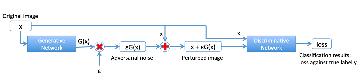
where l 𝑙 l is the cross-entropy loss, λ 𝜆 \lambda is the trade-off parameter between minimizing the loss on normal examples versus minimizing the loss on the adversarial examples, and ϵ italic-ϵ \epsilon is the magnitude of the noise. See Figure 1 for an illustration of the model.
In this work we focus on perturbations based on ℓ ∞ subscript ℓ \ell_ <\infty>norm. This can be achieved easily by adding a tanh layer as the final layer of the generator network G ϕ subscript 𝐺 italic-ϕ G_ <\phi>, which normalizes the output to the range of [ − 1 , 1 ] 1 1 [-1,1] . Perturbations based on ℓ 1 subscript ℓ 1 \ell_ or ℓ 2 subscript ℓ 2 \ell_ norms can be accommodated by having the appropriate normalization layers in the final layer of G ϕ subscript 𝐺 italic-ϕ G_ <\phi>.
We now explain the intuition of our approach. Ideally, we would like to find a solution θ 𝜃 \theta that has small risk on clean examples
| R ( θ ) = ∑ i = 1 n l ( D θ ( x i ) , y i ) , 𝑅 𝜃 superscript subscript 𝑖 1 𝑛 𝑙 subscript 𝐷 𝜃 subscript 𝑥 𝑖 subscript 𝑦 𝑖 R(\theta)=\sum_^l(D_(x_),y_), | (5) |
and also small risk on the adversarial examples under maximum perturbation of size ϵ italic-ϵ \epsilon
However, except for simple datasets like MNIST, there are usually fairly large differences between the solutions of R ( θ ) 𝑅 𝜃 R(\theta) and solutions of R a d v ( θ ) subscript 𝑅 𝑎 𝑑 𝑣 𝜃 R_(\theta) under the same model class D θ subscript 𝐷 𝜃 D_ (Tsipras et al., 2018) . Optimizing for the risk under white box attacks R a d v ( θ ) subscript 𝑅 𝑎 𝑑 𝑣 𝜃 R_(\theta) involves tradeoff on the risk on clean data R ( θ ) 𝑅 𝜃 R(\theta) . Note that R a d v ( θ ) subscript 𝑅 𝑎 𝑑 𝑣 𝜃 R_(\theta) represent the risk under white box attacks, since we are free to choose the perturbation Δ x Δ 𝑥 \Delta x with knowledge of θ 𝜃 \theta . This can be approximated using the powerful PGD attack.
Instead of allowing the perturbations Δ x Δ 𝑥 \Delta x to be completely free, we model the adversary as a neural network G ϕ subscript 𝐺 italic-ϕ G_ <\phi>with finite capacity
Here the adversarial noise G ϕ ( x i ) subscript 𝐺 italic-ϕ subscript 𝑥 𝑖 G_<\phi>(x_) is not allowed to directly depend on the discriminative network parameters θ 𝜃 \theta . Also, the generative network parameter ϕ italic-ϕ \phi is shared across all examples, not computed per example like Δ x Δ 𝑥 \Delta x . We believe this is closer to the situation of defending against black box attacks, when the adversary does not know the discriminator network parameters. However, we still want G ϕ subscript 𝐺 italic-ϕ G_ <\phi>to be expressive enough to represent powerful attacks, so that D θ subscript 𝐷 𝜃 D_ has a good adversary to train against. Previous work (Xiao et al., 2018; Baluja & Fischer, 2018) show that there are powerful classes of G ϕ subscript 𝐺 italic-ϕ G_ <\phi>that can attack trained classifiers D θ subscript 𝐷 𝜃 D_ effectively.
In traditional GANs we are most interested in the distributions learned by the generative network. The discriminative network is a helper that drives the training, but can be discarded afterwards. In our setting we are interested in both the discriminative network and the generative network. The generative network in our formulation can give us a powerful adversary for attacking, while the discriminative network can give us a robust classifier that can defend against adversarial noise.
The stability and convergence of GAN training is still an area of active research (Mescheder et al., 2018) . In this paper we adopt gradient regularization (Mescheder et al., 2017) to stabilize the gradient descent/ascent training. Denote the minimax objective in Eq. 4 as F ( θ , ϕ ) 𝐹 𝜃 italic-ϕ F(\theta,\phi) . With the generative network parameter fixed at ϕ k subscript italic-ϕ 𝑘 \phi_ , instead of minimizing the usual objective F ( θ , ϕ k ) 𝐹 𝜃 subscript italic-ϕ 𝑘 F(\theta,\phi_) to update θ 𝜃 \theta for the discriminator network, we instead try to minimize the regularized objective
where γ 𝛾 \gamma is the regularization parameter for gradient regularization. Minimizing the gradient norm ‖ ∇ ϕ F ( θ , ϕ k ) ‖ 2 superscript norm subscript ∇ italic-ϕ 𝐹 𝜃 subscript italic-ϕ 𝑘 2 \|\nabla_<\phi>F(\theta,\phi_)\|^ jointly makes sure that the norm of the gradient for ϕ italic-ϕ \phi at ϕ k subscript italic-ϕ 𝑘 \phi_ does not grow when we update θ 𝜃 \theta to reduce the objective F ( θ , ϕ k ) 𝐹 𝜃 subscript italic-ϕ 𝑘 F(\theta,\phi_) . This is important because if the gradient norm ‖ ∇ ϕ F ( θ , ϕ k ) ‖ 2 superscript norm subscript ∇ italic-ϕ 𝐹 𝜃 subscript italic-ϕ 𝑘 2 \|\nabla_<\phi>F(\theta,\phi_)\|^ becomes large after an update of θ 𝜃 \theta , it is easy to update ϕ italic-ϕ \phi to make the objective large again, leading to zigzagging behaviour and slow convergence. Note that the gradient norm term is zero at a saddle point according to the first-order optimality conditions, so the regularizer does not change the set of solutions. With these we update θ 𝜃 \theta using SGD with step size η D subscript 𝜂 𝐷 \eta_ :
𝑙 1 subscript 𝜃 𝑙 subscript 𝜂 𝐷 subscript ∇ 𝜃
𝐹 subscript 𝜃 𝑙 subscript italic-ϕ 𝑘
𝛾 2 superscript delimited-∥∥ subscript ∇ italic-ϕ 𝐹 subscript 𝜃 𝑙 subscript italic-ϕ 𝑘 2 subscript 𝜃 𝑙 subscript 𝜂 𝐷 delimited-[]
The Hessian-vector product term ∇ θ ϕ 2 F ( θ l , ϕ k ) ∇ ϕ F ( θ l , ϕ k ) subscript superscript ∇ 2 𝜃 italic-ϕ 𝐹 subscript 𝜃 𝑙 subscript italic-ϕ 𝑘 subscript ∇ italic-ϕ 𝐹 subscript 𝜃 𝑙 subscript italic-ϕ 𝑘 \nabla^_<\theta\phi>F(\theta_,\phi_)\nabla_<\phi>F(\theta_,\phi_) can be computed with double backpropagation provided by packages like Tensorflow/PyTorch, but we find it faster to compute it with finite difference approximation. Recall that for a function f ( x ) 𝑓 𝑥 f(x) with gradient g ( x ) 𝑔 𝑥 g(x) and Hessian H ( x ) 𝐻 𝑥 H(x) , the Hessian-vector product H ( x ) v 𝐻 𝑥 𝑣 H(x)v can be approximated by ( g ( x + h v ) − g ( x ) ) / h
𝑥 ℎ 𝑣 𝑔 𝑥 ℎ (g(x+hv)-g(x))/h for small h ℎ h (Pearlmutter, 1994) . Therefore we approximate:
where v = ∇ ϕ F ( θ l , ϕ k ) 𝑣 subscript ∇ italic-ϕ 𝐹 subscript 𝜃 𝑙 subscript italic-ϕ 𝑘 v=\nabla_<\phi>F(\theta_,\phi_) . Note that ϕ k + h v
subscript italic-ϕ 𝑘 ℎ 𝑣 \phi_+hv is exactly a gradient step for generative network G ϕ subscript 𝐺 italic-ϕ G_ <\phi>. Setting h ℎ h to be too small can lead to numerical instability. We therefore correlate h ℎ h with the gradient step size and set h = η G / 10 ℎ
subscript 𝜂 𝐺 10 h=\eta_
We update the generative network parameters ϕ italic-ϕ \phi with using (stochastic) gradient ascent. With the discriminative network parameters fixed at θ l subscript 𝜃 𝑙 \theta_ and step size η G subscript 𝜂 𝐺 \eta_ , we update:
We do not add a gradient regularization term for ϕ italic-ϕ \phi , since empirically we find that adding gradient regularization to θ 𝜃 \theta is sufficient to stabilize the training.
In the experiments we train both the discriminative network and generative network from scratch with random weight initializations. We do not need to pre-train the discriminative network with clean examples, or the generative network against some fixed discriminative networks, to arrive at good saddle point solutions.
In our experiments we find that the discriminative networks D θ subscript 𝐷 𝜃 D_ we use tend to overpower the generative network G ϕ subscript 𝐺 italic-ϕ G_ <\phi>if we just perform simultaneous parameter updates to both networks. This can lead to saddle point solutions where it seems G ϕ subscript 𝐺 italic-ϕ G_ <\phi>cannot be improved locally against D θ subscript 𝐷 𝜃 D_ , but in reality can be made more powerful by just running more gradient steps on ϕ italic-ϕ \phi . In other words we want the region around the saddle point solution to be relatively flat for G ϕ subscript 𝐺 italic-ϕ G_ <\phi>. To make the generative network more powerful so that the discriminative network has a good adversary to train against, we adopt the following strategy. For each update of θ 𝜃 \theta for D θ subscript 𝐷 𝜃 D_ , we perform multiple gradient steps on ϕ italic-ϕ \phi using the same mini-batch. This allows the generative network to learn to map the inputs in the mini-batch to adversarial noises with high loss directly, compared to running multiple gradient steps on different mini-batches. In the experiments we run 5 gradient steps on each mini-batch. We fix the tradeoff parameter λ 𝜆 \lambda (Eq. 4 ) over loss on clean examples and adversarial loss at 1. We also fix the gradient regularization parameter γ 𝛾 \gamma (Eq. 8 ) at 0.01, which works well for different datasets.
We implemented our adversarial network approach using Tensorflow (Abadi et al., 2016) , with the experiments run on several machines each with 4 GTX1080 Ti GPUs. In addition to our adversarial networks, we also train standard undefended models and models trained with adversarial training using PGD for comparison. For attacks we focus on the commonly used fast gradient sign (FGS) method, and the more powerful projected gradient descent (PGD) method.
For the fast gradient sign (FGS) attack, we compute the adversarial image by
where Proj X subscript Proj 𝑋 \text_ projects onto the feasible range of rescaled pixel values X 𝑋 X (e.g., [-1,1]).
For the projected gradient descent (PGD) attack, we iterate the fast gradient sign attack multiple times with projection, with random initialization near the starting point neighbourhood.
subscript 𝑥 𝑖 italic-ϵ 𝑢 superscript subscript ^ 𝑥 𝑖
𝑘 1 subscript Proj superscript subscript 𝐵 italic-ϵ subscript 𝑥 𝑖 𝑋
where u ∈ ℝ d 𝑢 superscript ℝ 𝑑 u\in\mathbb^ is a uniform random vector in [ − 1 , 1 ] d superscript 1 1 𝑑 [-1,1]^ , δ 𝛿 \delta is the step size, and B ϵ ∞ ( x i ) superscript subscript 𝐵 italic-ϵ subscript 𝑥 𝑖 B_^<\infty>(x_) is an ℓ ∞ subscript ℓ \ell_ <\infty>ball centered around the input x i subscript 𝑥 𝑖 x_ with radius ϵ italic-ϵ \epsilon . In the experiments we set δ 𝛿 \delta to be a quarter of the perturbation ϵ italic-ϵ \epsilon , i.e., ϵ / 4
italic-ϵ 4 \epsilon/4 , and the number of PGD steps k 𝑘 k to be 10. We adopt exactly the same PGD attack procedure when generating adversarial examples in PGD adversarial training. Our implementation is available at https://github.com/whxbergkamp/RobustDL_GAN.
For MNIST the inputs are black and white images of digits of size 28x28 with pixel values scaled between 0 and 1. We rescale the inputs to the range of [-1,1]. Following previous work (Kannan et al., 2018) , we study perturbations of ϵ = 0.3 italic-ϵ 0.3 \epsilon=0.3 (in the original scale of [0,1]). We use a simple convolutional neural network similar to LeNet5 as our discriminator networks for all training methods. For our adversarial approach we use an encoder-decoder network for the generator. See Model D1 and Model G0 in the Appendix for the details of these networks. We use SGD with learning rate of η D = 0.01 subscript 𝜂 𝐷 0.01 \eta_=0.01 and momentum 0.9, batch size of 64, and run for 200k iterations for all the discriminative networks. The learning rates are decreased by a factor of 10 after 100k iterations. We use SGD with a fixed learning rate η G = 0.01 subscript 𝜂 𝐺 0.01 \eta_=0.01 with momentum 0.9 for the generative network. We use weight decay of 1E-4 for standard and adversarial PGD training, and 1E-5 for our adversarial network approach (for both D θ subscript 𝐷 𝜃 D_ and G ϕ subscript 𝐺 italic-ϕ G_ <\phi>). For this dataset we find that we can improve the robustness of D θ subscript 𝐷 𝜃 D_ by running more updates on G ϕ subscript 𝐺 italic-ϕ G_ <\phi>, so we run 5 updates on G ϕ subscript 𝐺 italic-ϕ G_ <\phi>(each update contains 5 gradient steps described in Section 3.2 ) for each update on D θ subscript 𝐷 𝜃 D_ .
Table 1 (left) shows the white box attack accuracies of different models, under perturbations of ϵ = 0.3 italic-ϵ 0.3 \epsilon=0.3 for input pixel values between 0 and 1. Adversarial training with PGD performs best under white box attacks. Its accuracies stay above 90% under FGS and PGD attacks. Our adversarial network model performs much better than the undefended standard training model, but there is still a gap in accuracies compared to the PGD model. However, the PGD model has a small but noticeable drop in accuracy on clean examples compared to the standard model and adversarial network model.
Table 1 (right) shows the black box attack accuracies of different models. We generate the black box attack images by running the FGS and PGD attacks on surrogate models A’, B’ and C’. These surrogate models are trained in the same way as their counterparts (standard - A, PGD - B, adversarial network - C) with the same network architecture, but using a different random seed. We notice that the black box attacks tend to be the most effective on models trained with the same method (A’ on A, B’ on B, and C’ on C). Although adversarial PGD beats our adversarial network approach on white box attacks, they have comparable performance on these black box attacks. Interestingly, the adversarial examples from adversarial PGD (B’) and adversarial networks (C’) do not transfer well to the undefended standard model. The undefended model still have accuracies between 85-95%.
| conv2d(5,1,32) |
| maxpool(2) |
| conv2d(5,1,64) |
| maxpool(2) |
| FC(10) |
| conv2d(3,1,16) |
| residual-block(3,1,16) × 3 absent 3 \times 3 |
| residual-block(3,2,32) |
| residual-block(3,1,32) × 2 absent 2 \times 2 |
| residual-block(3,2,64) |
| residual-block(3,1,64) × 2 absent 2 \times 2 |
| avgpool(8) |
| FC(10) |